
Quadratic Assignment Problem: From Combinatorial Optimization to QUBO
Suppose you have a box full of LEGO blocks, and your task is to decide where each block should go. But as the number of blocks and possible positions grows, the number of possible arrangements grows rapidly. Finding the right arrangement becomes a problem of logical reasoning and optimization. Now replace those LEGO blocks with facilities, and the possible positions with a set of locations. Suddenly, the question becomes much more interesting: where should each facility be placed? This is where the Quadratic Assignment Problem, or QAP, enters. Unlike simply finding an available spot for each facility, QAP also considers how strongly the facilities interact with one another and how far apart their assigned locations are. The goal is to find an arrangement that minimizes the overall cost of these interactions. And this seemingly intuitive placement problem quickly turns into a challenging combinatorial optimization problem.
The difficulty comes from the fact that the cost of an assignment depends not only on the individual locations of facilities, but also on the interaction between pairs of facilities. This makes QAP a natural example for exploring how a practical optimization problem can be translated into a Quadratic Unconstrained Binary Optimization (QUBO) problem and then used in a quantum optimization workflow.
Understanding the Quadratic Assignment Problem
Consider three facilities: A, B and C and three possible locations: 1, 2 and 3. The facilities interact with one another. For example, facility A may exchange material frequently with facility B, while A and C may interact less frequently. These interactions is represented by the Flow matrix F. Similarly the locations have distances between them, represented by a distance matrix D.
The objective is therefore to find an assignment that minimizes the total interaction cost, where each facility-to-facility flow is weighted by the distance between their assigned locations. This structure appears in problems such as facility layout, warehouse design, electronic design, logistics, and resource allocation. To explore standard historical benchmarks and data sets for these applications, researchers often rely on QAPLIB.
Encoding the Assignment Problem
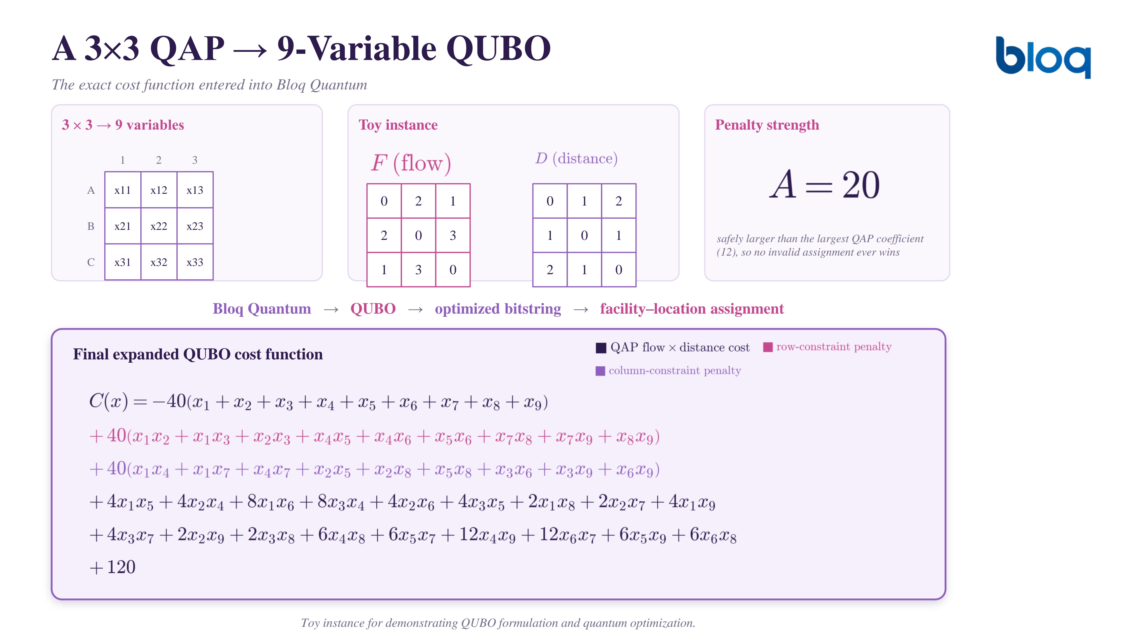
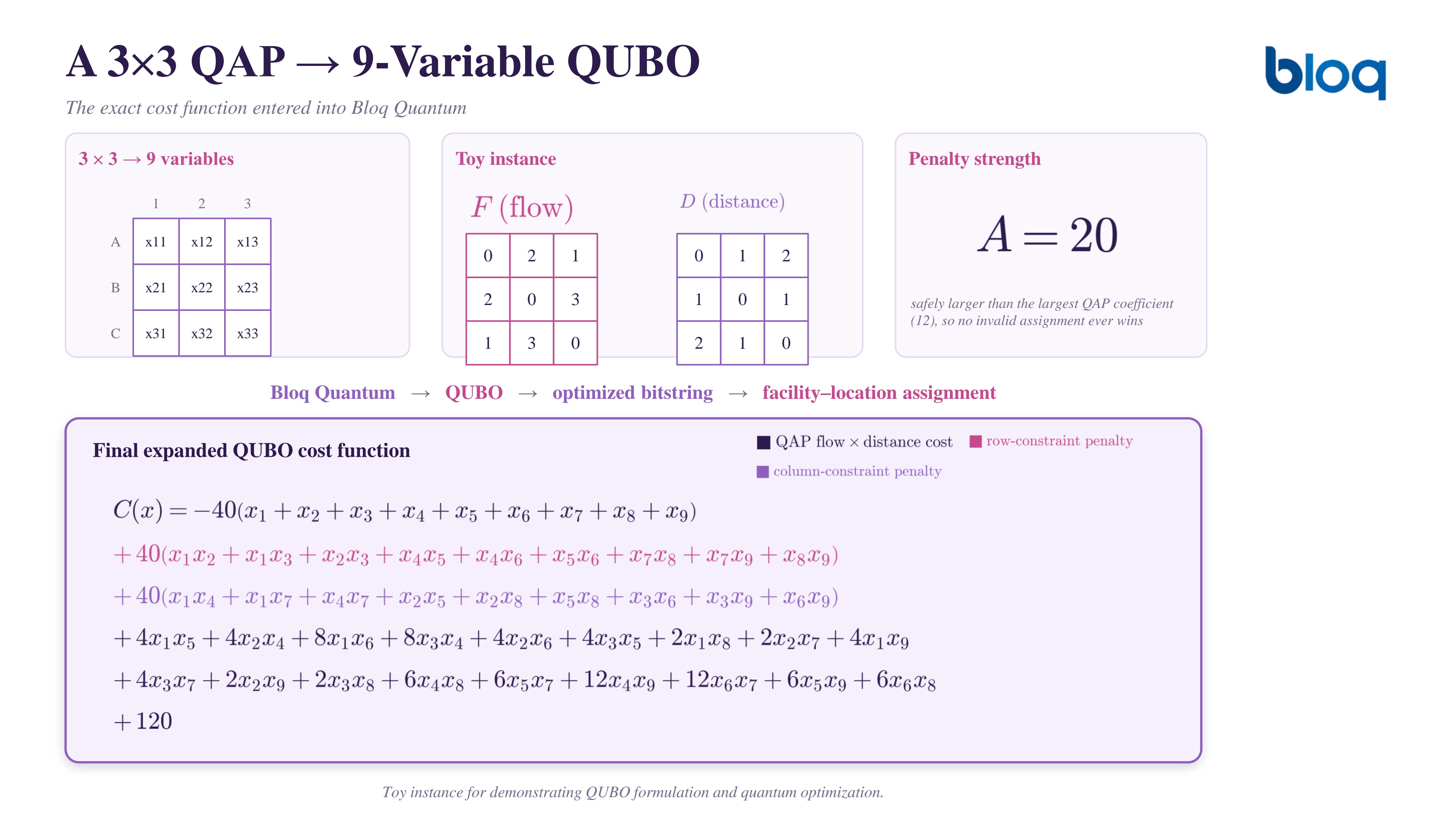
Once we have defined the facilities and locations, we need a way to represent a particular assignment mathematically. For this, we introduce a binary variable for every possible facility–location pair. A variable is set to 1 when a facility is assigned to a particular location, and 0 otherwise. For three facilities and three locations, this gives us nine binary variables, which can be arranged as a 3 × 3 assignment grid. The original QAP objective then combines two pieces of information: the interaction between a pair of facilities and the distance between the locations assigned to them. In other words, every possible pair of assignments contributes a cost based on how strongly those facilities interact and how far apart their assigned locations are. This is what gives QAP its quadratic structure. The cost depends on pairs of binary variables rather than on individual variables alone. However, there is one more thing we need to take care of. Simply minimizing this quadratic cost does not guarantee that we get a valid assignment. We need to ensure that each facility is assigned to exactly one location, and each location receives exactly one facility.
This is where the QUBO formulation comes in. We incorporate these assignment requirements as penalty terms, so that solutions violating the constraints receive an additional cost. The resulting expression is an unconstrained binary optimization problem that can be represented as a QUBO and passed to a quantum optimization workflow. For a deeper mathematical dive into mapping objective functions and constraints, resources like the Tutorial on Formulating and Using QUBO Models or the D-Wave Problem Formulation Guide offer comprehensive step-by-step techniques
Turning the QAP into a QUBO
For our example, we now consider three facilities and three possible locations. Since every facility can potentially be assigned to every location, there are nine possible facility-location assignments. We represent each of these assignments using a binary variable, giving us a total of nine variables.
The QAP objective and the one-to-one assignment requirements are then combined into a single quadratic cost function. The assignment requirements are incorporated using penalty terms, with a penalty strength of 20 in our example. This ensures that the optimization problem accounts not only for the interaction and distance costs, but also for whether a proposed assignment satisfies the required constraints. After expanding the formulation, we obtain the final QUBO expression for our nine binary variables. This is the expression that we enter into Bloq Quantum. From here, the workflow is straightforward: we provide the QUBO to Bloq, run the optimization, and obtain a binary string as the output. We can then map the bits of this string back to our 3 × 3 assignment grid to interpret which facility-location combinations have been selected.
Implementing the QUBO in Bloq Quantum
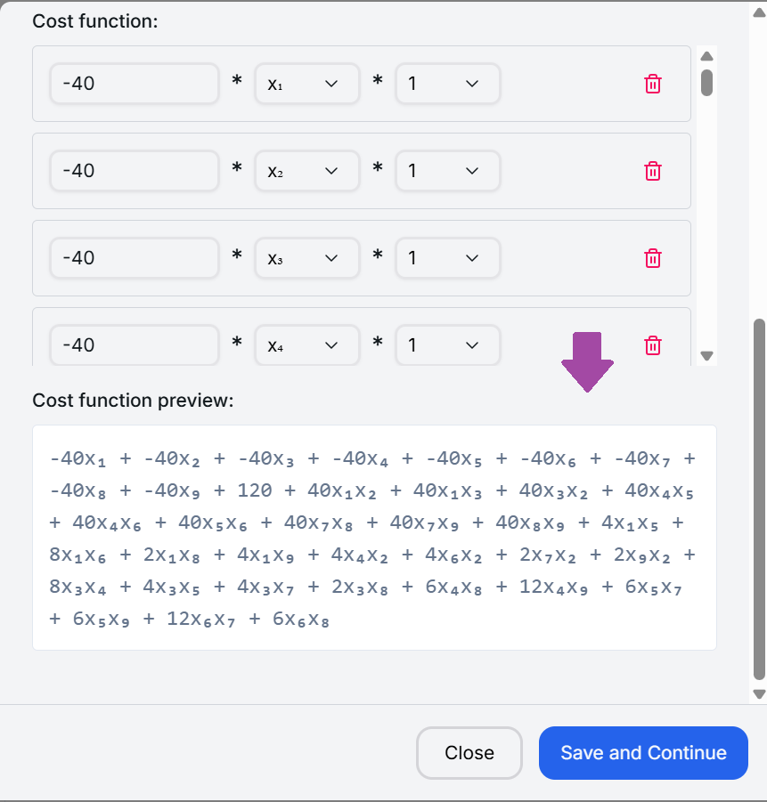
With the QUBO formulation ready, we can now move from the mathematical model to the actual optimization workflow. The expanded QUBO expression from the previous section is entered directly into Bloq Quantum. Each binary variable represents one possible facility-location assignment, and the optimizer searches through the corresponding binary states to evaluate the objective function. For our 3 × 3 example, the optimization produces a binary string representing one of the candidate states explored by the solver. We can then split this string into three groups of three bits and map them back onto our assignment grid.
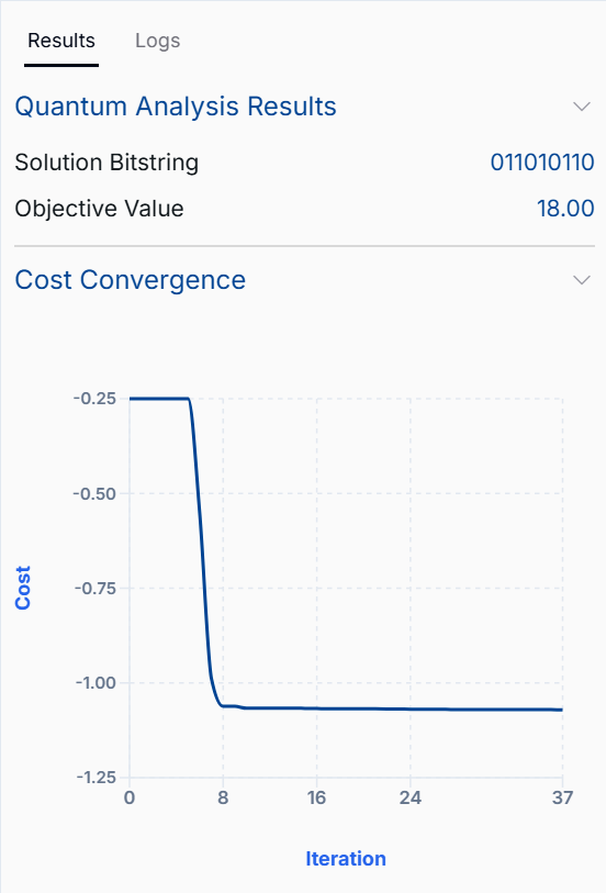
For example, the output from our run is the bitstring 011010110, with an objective value of 18. Reading the bits according to the assignment-variable ordering allows us to translate the numerical output back into the original facility-location problem. This step is important because the bitstring is not just an abstract collection of zeros and ones. It is the encoded representation of a possible solution to the original QAP.
Conclusion
The Quadratic Assignment Problem is a simple idea with a surprisingly difficult optimization landscape. Once the number of facilities and locations grows, the number of possible assignments increases rapidly, making an exhaustive search impractical.
In this walkthrough, we started with the basic QAP formulation and represented the facility-location decisions using binary variables. We then incorporated the one-to-one assignment requirements through penalty terms and transformed the problem into a QUBO. For our small 3 × 3 example, this resulted in a nine-variable QUBO that could be entered directly into Bloq Quantum. The resulting bitstring shows how a solution to the binary optimization problem can be mapped back to the original facility-location problem.
A real-world placement problem can be expressed as a mathematical optimization problem, transformed into a QUBO, and then passed into a quantum optimization workflow.This QAP example is small enough to understand by hand, but the same formulation approach provides a foundation for exploring larger and more complex combinatorial optimization problems with quantum computing ecosystems like the Qiskit Optimization Module and PennyLane.